When researchers don't understand how a model works, they struggle to incorporate their findings into the larger knowledge landscape. Similarly, interpretability becomes essential when trying to identify bias or troubleshoot algorithmic errors. As algorithms increasingly influence our society, comprehending exactly how they generate their outputs becomes more critical than ever. Though several important model-agnostic interpretability methods exist, none are perfect—yet they remain valuable tools for interpreting even highly complex machine learning models.
In this article, we'll examine why popular interpretability techniques can be misleading despite their widespread use. We'll analyze the limitations of methods like Partial Dependence Plots, ICE plots, surrogate models, and SHAP values, while providing guidance on how to choose and validate the right interpretability approach for your specific needs.
Why Interpretability Techniques Can Be Misleading
Interpreting complex machine learning models presents significant challenges for data scientists. The techniques we rely on to peek inside these black boxes can lead us astray if we're not careful. Let's examine the primary ways interpretation methods might mislead us.
Over-reliance on visualizations without statistical grounding
Visualizations serve as powerful tools for understanding model behavior, but they aren't without risks. The main danger lies in the potential misinterpretation of graphic representations. Poorly designed visualizations can mislead users and cause misunderstandings, especially when they lack a statistical foundation.
Several studies have found that visualizations without adequate statistical grounding fail to create correct representations of the actual data, consequently leading to wrong perception, interpretation, and ultimately flawed decisions. Furthermore, visualization places the burden of discovery on the user, making it susceptible to confirmation bias – we often see what we're conditioned to see and miss breakthrough evidence.
Visualization tools also face practical limitations. They typically represent only two or three dimensions before becoming overwhelming. This constraint becomes particularly problematic when analyzing high-dimensional data, where relationships between multiple features cannot be adequately captured in simplified visual formats.
Assuming feature independence in correlated datasets
Many interpretability methods operate under the assumption that features are independent – an assumption frequently violated in real-world datasets. When features are dependent, perturbation-based techniques like Permutation Feature Importance (PFI), Partial Dependence Plots (PDP), LIME, and Shapley values can produce misleading results.
The primary issue occurs during the perturbation process, where these methods:
- Produce unrealistic data points located outside the multivariate joint distribution
- Sever both the connection to the target variable and the interdependence with correlated features
- Generate artificial data points that may never occur in reality
For instance, in a model predicting heart attack risk, features like "weight yesterday" and "weight today" would be highly correlated. During perturbation, the PFI method might shuffle one feature while leaving the other unchanged, creating impossible combinations. This leads to evaluating the model in areas of the feature space with little or no observed data, where model uncertainty is exceptionally high.
Ignoring model-specific behavior in model-agnostic tools
Model-agnostic methods provide flexibility across different model types but can fail to capture important model-specific nuances. These tools typically condense the complexity of ML models into human-intelligible descriptions that only provide insight into specific aspects of the model and data.
Different interpretation methods measure different aspects of feature relevance. For example, the relevance measured by PFI can differ significantly from the relevance measured by SHAP importance.
Consequently, applying an interpretability method designed for one purpose in an unsuitable context leads to misleading conclusions.
Additionally, most model-agnostic methods provide additive explanations without separating main effects from interactions. They may not adequately account for how different parts of the model work together, particularly in architectures with complex internal representations.
For interpretations to be valid, both the original model and any secondary analysis must accurately capture the data-generating process. If a deep learning model fits the data well but a post hoc analysis with LIME doesn't sufficiently capture the original model's behavior, the resulting interpretations will be inaccurate.
By understanding these limitations, we can approach model interpretability techniques with appropriate caution and select methods that match our specific analytical needs.
Limitations of Popular Model Interpretability Techniques

Popular interpretability methods come with significant limitations that can undermine their effectiveness. Understanding these constraints is essential for applying these techniques appropriately and avoiding misleading conclusions.
Partial Dependence Plots (PDP) and hidden heterogeneity
PDPs operate at an aggregated level, averaging all data points to create a single curve that shows the marginal effect of a feature on model predictions. This aggregation, nevertheless, can hide important differences across subpopulations. In cases where predictions increase for half the population and decrease for the other half when a feature value changes, the averaged PDP curve might incorrectly show no effect at all.
The effectiveness of PDPs diminishes in several situations:
- When analyzing sparse data regions, PDPs become untrustworthy as they may generalize from too few observations
- PDPs assume feature independence, yet in real-world datasets, features are often correlated
- Heterogeneous effects remain hidden because PDPs only show average marginal effects
In essence, PDP assumes that features for which partial dependence is computed are not correlated with other features. When this assumption is violated—which happens frequently in practice—PDPs create unrealistic data points during the perturbation process. For instance, a PDP might generate combinations like extreme temperature values in seasons where they never occur naturally.
ICE plots and misleading individual trends
Individual Conditional Expectation (ICE) plots were developed to address PDPs' inability to reveal heterogeneous effects. Rather than showing only the average effect, ICE plots display individual prediction trajectories for each observation separately. Initially, this appears to solve the heterogeneity problem.
Subsequently, ICE plots introduce their own limitations. They can only meaningfully display one feature at a time, as two features would require overlapping surfaces that become visually incomprehensible. Moreover, with many observations, plots become overcrowded and difficult to interpret.
ICE plots likewise suffer from the correlation problem. When the feature of interest correlates with other features, some points in the plotted lines might represent invalid data points according to the joint feature distribution. Accordingly, the curves may display predictions for impossible combinations of feature values, leading to unreliable interpretations.
Additionally, ICE curves still may not adequately reveal interaction effects, primarily when interactions are continuous and curves start at different intercepts. In such cases, derivative or centered ICE curves, which eliminate differences in intercepts, might provide better insights.
Permuted Feature Importance and instability with correlated features
Permutation Feature Importance (PFI) measures a feature's importance by calculating the increase in model prediction error after permuting the feature values. Essentially, this breaks the relationship between the feature and the target variable.
The permutation approach faces serious challenges with correlated features. When features correlate, permuting one feature not only breaks its association with the target variable but also disrupts its relationship with correlated features. This creates unrealistic data instances ranging from unlikely to impossible combinations.
Furthermore, adding correlated features to a dataset can lead to a decrease in measured feature importance. For example, in a model predicting heart attack risk using a person's weight from yesterday and today (highly correlated features), the importance splits between both features since either provides similar predictive value.
PFI also exhibits instability with correlated features. Different permutations of the same feature can produce varying importance scores, creating inconsistent rankings. This instability becomes especially problematic in high-dimensional datasets with complex dependency structures.
Coupled with these issues, PFI may deem features of low importance for poorly performing models, even if those same features would be crucial in better models. This highlights the fact that permutation importance reflects feature importance for a specific model rather than the intrinsic predictive value of a feature.
Surrogate Models: When Simplicity Fails

Surrogate models promise simplicity and interpretability by approximating complex black-box models with more transparent alternatives. Yet, these simplified representations often fall short in critical ways that can lead to misinterpretation and flawed conclusions.
Global Surrogates and loss of fidelity
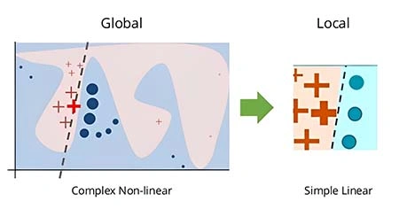
Global surrogate models attempt to approximate an entire black-box model with a simpler, interpretable alternative. Unfortunately, this approach suffers from fundamental limitations. First, surrogates are models trained on another model's outputs rather than actual observations, meaning they can "stray farther from the real-world and lose predictive power". This loss of fidelity becomes particularly apparent when evaluating out-of-distribution data.
Research has identified consistent "generalization gaps" where simplified proxies accurately approximate the original model on in-distribution evaluations but fail on tests of systematic generalization. In some cases, the surrogate underestimates the original model's generalization capabilities, while in others, it unexpectedly outperforms the original model—both scenarios indicate a concerning mismatch between the original and its simplification.
Additionally, surrogate models often perform inconsistently across different data subsets, closely approximating results for one segment while producing inaccurate results for another. This partial interpretability creates a false sense of understanding that may be more dangerous than acknowledged ignorance.
LIME and the problem of local instability
LIME (Local Interpretable Model-Agnostic Explanations) encounters a significant challenge: explanation instability. Notably, when LIME is run multiple times on the same individual with identical parameters, it frequently produces entirely different explanations. This inconsistency stems primarily from LIME's generation step, which creates random datasets for each call, resulting in different underlying linear models.
The instability issue undermines trust in both the explanation method and, by extension, the original model itself. As one researcher notes, "unstable LIME explanations are a real pain and can generate distrust in the entire Machine Learning field". Technical analysis attributes this instability to several factors, including "tokenization variance, perturbation sampling noise, and local non-linearity of the decision surface".
Sampling bias in perturbed instances
The sampling process in surrogate models introduces substantial bias, specifically when generating perturbed instances. LIME, in particular, "samples from a Gaussian distribution, ignoring the correlation between features". This approach "can lead to unlikely data points" that don't represent realistic scenarios.
To illustrate, consider a banking model that uses correlated financial indicators. When LIME perturbs these features independently, it creates impossible combinations—like customers with high savings but severe debt—forcing the model to make predictions on scenarios that would never occur naturally.
Given these limitations, surrogate models should be applied with extreme caution, particularly in high-stakes domains. To improve reliability, researchers have developed stability indices like VSI (Variables Stability Index) and CSI (Coefficients Stability Index) to measure consistency across multiple LIME explanations, enabling more careful validation before deployment in critical applications.
SHAP Values: Theoretical Strengths vs Practical Pitfalls

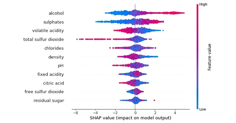
SHAP values, rooted in game theory, have become a cornerstone of model interpretability techniques due to their mathematical foundation. Yet, beneath their theoretical elegance lie significant practical challenges that limit their effectiveness.
Computational cost in large datasets
SHAP calculations face exponential computational complexity—for a model with n features, exact computation requires evaluating 2^n possible feature subsets. This renders exact calculations infeasible for high-dimensional data. Processing explanations for 20 million instances in a random forest with 400 trees and depth capped at 12 can take up to 15 hours, even on a machine equipped with 100 cores.
Hence, various approximation methods have emerged:
- KernelSHAP: Uses dataset sampling, but becomes intractable when features exceed ten
- TreeSHAP: Reduces complexity to O(TLD²) where T is tree count, L is leaf count, and D is depth
- Fast TreeSHAP: Further optimizes to O(TL²D + MTLD) time complexity
These approximations markedly improve performance but inevitably introduce trade-offs between accuracy and speed.
Misinterpretation of additive contributions
Fundamentally, SHAP values assume additive feature contributions, which can produce misleading interpretations. The method struggles with:
- Strong interaction effects between features that aren't captured by individual attribution values
- Correlated features leading to imprecise values—even correlations as low as 0.2 can cause significant deviations
- Instances where irrelevant features receive non-zero scores while relevant features get zero scores
One study concluded that "SHAP exhibits important limitations as a tool for measuring feature importance", highlighting that approximations rarely match exact SHAP scores, especially in models with numerous features.
Dependence on background data distribution
The stability of SHAP explanations depends heavily on the background dataset used. Generally, this dataset consists of instances randomly sampled from training data. Ultimately, changing the background dataset alters the SHAP values—an often overlooked weakness.
Research demonstrates that explanation fluctuations decrease as background dataset size increases. The official SHAP documentation suggests 100 random samples, yet this recommendation conflicts with other studies using different sampling sizes. Users should consider the computational complexity tradeoff: with m background samples, complexity increases linearly by m/100 × C₁₀₀.
Overall, while SHAP offers theoretical guarantees, practical implementations require careful validation to avoid drawing misleading conclusions from compromised results.
How to Choose and Validate Interpretability Methods
Selecting the right interpretability approach requires thoughtful matching between your specific use case and evaluation method. The choice ultimately determines whether your interpretability efforts yield valuable insights or misleading conclusions.
Global vs Local: Matching method to use case
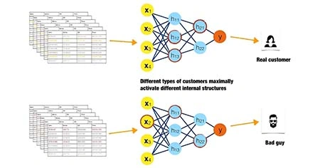
The distinction between global and local explainability shapes which technique best fits your needs. Global methods reveal consistent patterns across thousands of predictions, offering insights into overall model behavior. Conversely, local methods pinpoint reasons for specific outcomes with greater precision. When deciding between them, consider starting with global methods to evaluate whether the model aligns with domain knowledge, then applying local methods for edge cases or exceptions that require deeper investigation. This two-step approach prevents missing key nuances that global averages might conceal.
Functionally grounded vs human-grounded evaluation
Evaluating interpretability techniques falls into three categories: application-grounded, human-grounded, and functionally grounded. Application-grounded evaluation involves domain experts testing explanations in real-world settings. Meanwhile, human-grounded evaluation uses simpler experiments with non-experts to assess explanation quality. Functionally-grounded approaches offer the advantage of not requiring human experiments, instead using proxies for explanation quality. For instance, if users understand decision trees well, tree depth might serve as a proxy for explanation quality. Choose your evaluation method based on available resources and specific needs—application-grounded approaches provide the most realistic assessment but require more time and expertise.
Avoiding over-interpretation in high-stakes decisions
High-stakes decisions involve large potential losses and high reversal costs. Unfortunately, studies show that 78% of subjects fail to seek probability information when evaluating risky decisions. This becomes problematic with interpretability techniques that might oversimplify complex models. To avoid over-interpretation, match your method to user expertise—domain experts may prefer sophisticated explanations while others might need simpler ones. Additionally, consider time constraints—quick decisions may require easily understood explanations, whereas less time-sensitive scenarios allow for more comprehensive analysis. Finally, regularly validate interpretations through cross-validation techniques to ensure they remain reliable across different data subsets.
Conclusion
Throughout this analysis, we've examined how model interpretability techniques, despite their widespread adoption, can lead researchers astray when not properly understood. Certainly, these methods offer valuable insights into complex models, though they come with significant limitations that deserve careful consideration.
Partial Dependence Plots struggle with correlated features and mask heterogeneous effects. Individual Conditional Expectation plots, while addressing some PDP shortcomings, create their own visualization challenges and still suffer from correlation issues. Surrogate models promise simplicity but often sacrifice critical fidelity to the original model. Even SHAP values, with their strong theoretical foundation, face practical implementation challenges that can compromise their reliability.
Undoubtedly, the limitations we've explored underscore a fundamental truth: no single interpretability technique provides a complete picture. Rather than relying exclusively on one method, researchers should employ multiple complementary approaches while remaining cognizant of their respective weaknesses. Additionally, validation across different data subsets and sensitivity analysis help ensure robust interpretations.
The stakes for proper model interpretation continue to rise as machine learning increasingly influences critical decisions across healthcare, finance, and criminal justice. Therefore, responsibility falls on practitioners to verify their interpretations through rigorous testing before drawing conclusions that might affect real lives.
Last but not least, we must acknowledge that interpretability itself remains an evolving field. The techniques available today represent early attempts at cracking open the black box of complex models. As research advances, we expect more sophisticated methods that address current limitations while providing deeper insights into model behavior.
By approaching model interpretation with appropriate skepticism and methodological rigor, we can extract genuine insights from our models without falling victim to misleading explanations or false confidence in our understanding.
FAQs
Q1. What are some common pitfalls of model interpretability techniques?
Some common pitfalls include over-relying on visualizations without statistical grounding, assuming feature independence in correlated datasets, and ignoring model-specific behavior when using model-agnostic tools. These can lead to misleading or incomplete explanations of model behavior.
Q2. Why are surrogate models sometimes problematic for interpretability?
Surrogate models can lose fidelity to the original complex model, suffer from local instability in their explanations, and introduce sampling bias when generating perturbed instances. This can result in oversimplified or inaccurate interpretations of the original model's decision-making process.
Q3. What are the main challenges with using SHAP values for model interpretation?
Key challenges include high computational costs for large datasets, potential misinterpretation of additive feature contributions, and dependence on the background data distribution. These factors can impact the reliability and practicality of SHAP-based explanations.
Q4. How should one choose between global and local interpretability methods?
The choice depends on the specific use case. Global methods reveal overall model behavior and are useful for evaluating alignment with domain knowledge. Local methods provide more precise explanations for individual predictions and are better for investigating edge cases or exceptions.
Q5. What steps can be taken to avoid over-interpretation in high-stakes decisions?


